Logistic Regression#
0. Introduction#
This notebook follows after the “General Linear Model.iypnb” notebook. Aim of this notebook is to conduct the logistic regression algorithm. For now, we have 26 z-maps, so one for each contrast, for each session, per run i.e. 4 * 5 * 26 z-maps.
1. Masking#
First we will need to load the mask. The masks needs to be fetched from the openneuro dataset. This is done with datalad.
We cd into the local dataset directory and then use the command:
datalad get sourcedata/sub-01/anat.
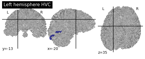
The masks are bi-lateral organised, meaning one mask per hemisphere. For starters, ventral portion of the v1 cortex in the left hemisphere (LH_V1v) will be the first mask.
import os

os.chdir("/home/jpauli/ds001506/sourcedata/sub-01/anat")
os.listdir()
['sub-01_mask_LH_FFA.nii.gz',
 'sub-01_mask_LH_hV4.nii.gz',
 'sub-01_mask_LH_HVC.nii.gz',
 'sub-01_mask_LH_LOC.nii.gz',
 'sub-01_mask_LH_PPA.nii.gz',
 'sub-01_mask_LH_V1d.nii.gz',
 'sub-01_mask_LH_V1v.nii.gz',
 'sub-01_mask_LH_V2d.nii.gz',
 'sub-01_mask_LH_V2v.nii.gz',
 'sub-01_mask_LH_V3d.nii.gz',
 'sub-01_mask_LH_V3v.nii.gz',
 'sub-01_mask_RH_FFA.nii.gz',
 'sub-01_mask_RH_hV4.nii.gz',
 'sub-01_mask_RH_HVC.nii.gz',
 'sub-01_mask_RH_LOC.nii.gz',
 'sub-01_mask_RH_PPA.nii.gz',
 'sub-01_mask_RH_V1d.nii.gz',
 'sub-01_mask_RH_V1v.nii.gz',
 'sub-01_mask_RH_V2d.nii.gz',
 'sub-01_mask_RH_V2v.nii.gz',
 'sub-01_mask_RH_V3d.nii.gz',
 'sub-01_mask_RH_V3v.nii.gz']
len(os.listdir())
22
We can see that there are 22 masks in total, 11 for each hemisphere.
mask_img_path = '/home/jpauli/ds001506/sourcedata/sub-01/anat'
mask_img_L = os.path.join(mask_img_path,'sub-01_mask_LH_V1v.nii.gz')
As mentioned before in the literature review part, The V1 seems to be a suitable canidate for mental imagery. Thus, we will choose this region as our mask.
This mask can also be plotted with respect to the z-map.
func_filename_path = '/mnt/c/Users/janos/git/sessions_new/z_maps_1_perrun'
func_filename =  os.path.join(func_filename_path,'01_active -1443537.0_1_z_map.nii.gz')
coordinates_func = (-20,-13,35)
from nilearn.plotting import plot_roi
plot_roi(mask_img_L, func_filename,display_mode='ortho',cut_coords=coordinates_func,
         title="Left hemisphere HVC")
/home/jpauli/miniconda3/envs/neuro_ai/lib/python3.7/site-packages/numpy/ma/core.py:2830: UserWarning: Warning: converting a masked element to nan.
  order=order, subok=True, ndmin=ndmin)
<nilearn.plotting.displays._slicers.OrthoSlicer at 0x7fda15e767b8>
Now the next step is to load in the X and y variables. We will do this by applying Nilearns Niftimasker function on the z-maps we calculated.
from nilearn.maskers import NiftiMasker
nifti_masker = NiftiMasker(mask_img=mask_img_L)
This loops helps us in extracting the voxel pattern from each z-map. Also, we append values to the y list. We have 26 different categories we want to decode. Since there are 4 sessions in total and the categories are the same for each session, we will add a “1” for category one and so on to the y list.
Since there are 5 runs per category, we also need to define a category starting index and a boundary index. This way we can keep track of which z-maps belongs to which image category.
X = []
y = []
Sessions = []
category = 1
cat_index = 0
cat_index_boundary = 5
for session in ["1","2","3","4"]:
    os.chdir('/mnt/c/Users/janos/git/sessions_new/z_maps_{}_perrun'.format(session))
    for x in os.listdir():
        if x == 'nilearn_cache':
            continue
        else:
            X.append(nifti_masker.fit_transform(x))
            y.append(category)
            Sessions.append(session)
            cat_index = cat_index + 1
            if cat_index == cat_index_boundary:
                category=category+1
                cat_index_boundary = cat_index_boundary+5
            if category == 27:
                category = 1
First we need to transform our list type variables into numpy arrays. Then, we can check the shape of our input (X) and output (y) data.
import numpy as np
y = np.array(y)
y.shape
y.shape
(520,)
import pandas as pd
df =  pd.DataFrame(np.concatenate(X))
X = df.to_numpy()
X.shape
(520, 992)
There are 520 rows for both X and y. This makes sense, because each row represents the respective image category label. The columns in our X data represents the voxels in our specific mask, in other words: We have the activity of 992 voxels per category.
2.0 Correlation matrix and voxel pattern#
The shape of our input array X tells us, that we have n_samples = 520 and n_features = 992. The features relate to the amount of voxels extracted. The samples are the 26 categories multiplied by all 4 sessions and all 5 runs per session.
First, we will take a look at the correlation matrix.
import matplotlib.pyplot as plt
corr =np.corrcoef(X)
plt.matshow(corr, cmap='coolwarm')
plt.colorbar()
plt.xlabel('Samples')
plt.ylabel('Samples')
Text(0, 0.5, 'Samples')
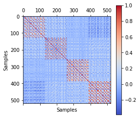
The correlation matrix tells us, that there are 4 large patterns to detect. The correlation patterns are between each session. This means, that there is a huge correlation within each session, but not between sessions. This could lead to some problems later on. We will first examine the voxel pattern, run the logist regression model and then see, how much the correlation will affect our results.
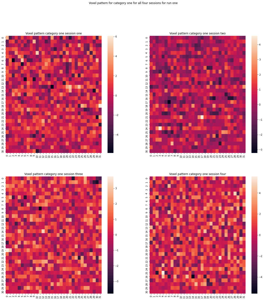
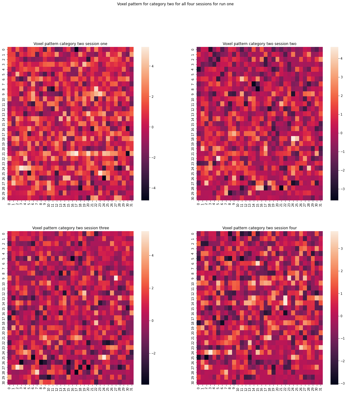
We now want to examine the voxel pattern for different given categories and sessions. This can help with understanding the data we are dealing with.
X_1 = np.reshape(X[0],(31,32))
X_11 = np.reshape(X[130],(31,32))
X_12 = np.reshape(X[260],(31,32))
X_13 = np.reshape(X[390],(31,32))


X_2 = np.reshape(X[1],(31,32))
X_21 = np.reshape(X[131],(31,32))
X_22 = np.reshape(X[261],(31,32))
X_23 = np.reshape(X[391],(31,32))

X_3 = np.reshape(X[2],(31,32))
X_31 = np.reshape(X[132],(31,32))
X_32 = np.reshape(X[262],(31,32))
X_33 = np.reshape(X[392],(31,32))

X_4 = np.reshape(X[3],(31,32))
X_41 = np.reshape(X[133],(31,32))
X_42 = np.reshape(X[263],(31,32))
X_43 = np.reshape(X[393],(31,32))
import seaborn as sns
figure, axis = plt.subplots(2, 2,figsize=(20, 20))
im1 = sns.heatmap(X_1,ax=axis[0,0])
im2= sns.heatmap(X_11,ax=axis[0,1])
im3= sns.heatmap(X_12,ax=axis[1,0])
im4= sns.heatmap(X_13, ax=axis[1,1])

#figure.colorbar(orientation='vertical')
axis[0, 0].set_title("Voxel pattern category one session one")
axis[0, 1].set_title("Voxel pattern category one session two")
axis[1, 0].set_title("Voxel pattern category one session three")
axis[1, 1].set_title("Voxel pattern category one session four")

figure.suptitle('Voxel pattern for category one for all four sessions for run one')
Text(0.5, 0.98, 'Voxel pattern for category one for all four sessions for run one')
figure, axis = plt.subplots(2, 2,figsize=(20, 20))
im1 = sns.heatmap(X_2,ax=axis[0,0])
im2= sns.heatmap(X_21,ax=axis[0,1])
im3= sns.heatmap(X_22,ax=axis[1,0])
im4= sns.heatmap(X_23, ax=axis[1,1])

#figure.colorbar(orientation='vertical')
axis[0, 0].set_title("Voxel pattern category two session one")
axis[0, 1].set_title("Voxel pattern category two session two")
axis[1, 0].set_title("Voxel pattern category two session three")
axis[1, 1].set_title("Voxel pattern category two session four")

figure.suptitle('Voxel pattern for category two for all four sessions for run one')
Text(0.5, 0.98, 'Voxel pattern for category two for all four sessions for run one')
figure, axis = plt.subplots(2, 2,figsize=(20, 20))
im1 = sns.heatmap(X_3,ax=axis[0,0])
im2= sns.heatmap(X_31,ax=axis[0,1])
im3= sns.heatmap(X_32,ax=axis[1,0])
im4= sns.heatmap(X_33, ax=axis[1,1])
#figure.colorbar(orientation='vertical')
axis[0, 0].set_title("Voxel pattern category three session one")
axis[0, 1].set_title("Voxel pattern category three session two")
axis[1, 0].set_title("Voxel pattern category three session three")
axis[1, 1].set_title("Voxel pattern category three session four")
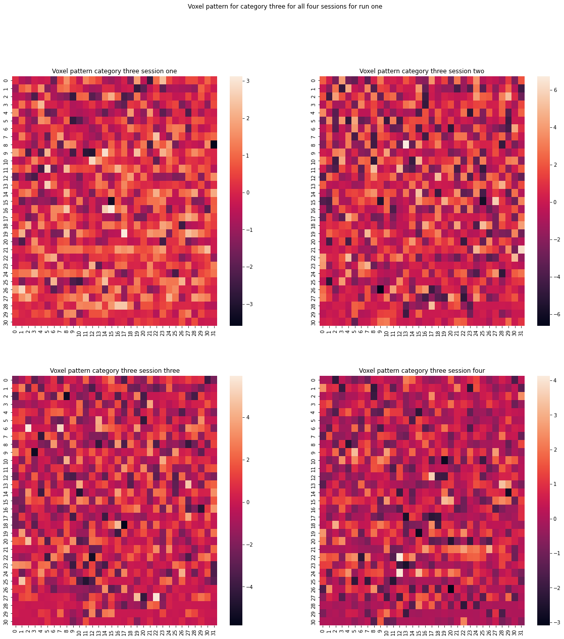
figure.suptitle('Voxel pattern for category three for all four sessions for run one')
Text(0.5, 0.98, 'Voxel pattern for category three for all four sessions for run one')
figure, axis = plt.subplots(2, 2,figsize=(20, 20))
im1 = sns.heatmap(X_4,ax=axis[0,0])
im2= sns.heatmap(X_41,ax=axis[0,1])
im3= sns.heatmap(X_42,ax=axis[1,0])
im4= sns.heatmap(X_43, ax=axis[1,1])
#figure.colorbar(orientation='vertical')
axis[0, 0].set_title("Voxel pattern category four session one")
axis[0, 1].set_title("Voxel pattern category four session two")
axis[1, 0].set_title("Voxel pattern category four session three")
axis[1, 1].set_title("Voxel pattern category four session four")
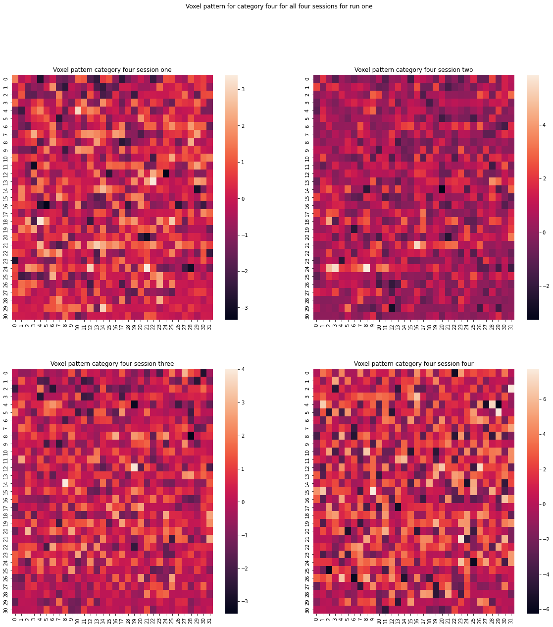
figure.suptitle('Voxel pattern for category four for all four sessions for run one')
Text(0.5, 0.98, 'Voxel pattern for category four for all four sessions for run one')
figure, axis = plt.subplots(2, 2,figsize=(20, 20))
im1 = sns.heatmap(X_1,ax=axis[0,0])
im2= sns.heatmap(X_2,ax=axis[0,1])
im3= sns.heatmap(X_3,ax=axis[1,0])
im4= sns.heatmap(X_4, ax=axis[1,1])
#figure.colorbar(orientation='vertical')
axis[0, 0].set_title("Voxel pattern category one session one")
axis[0, 1].set_title("Voxel pattern category two session one")
axis[1, 0].set_title("Voxel pattern category three session one")
axis[1, 1].set_title("Voxel pattern category four session one")
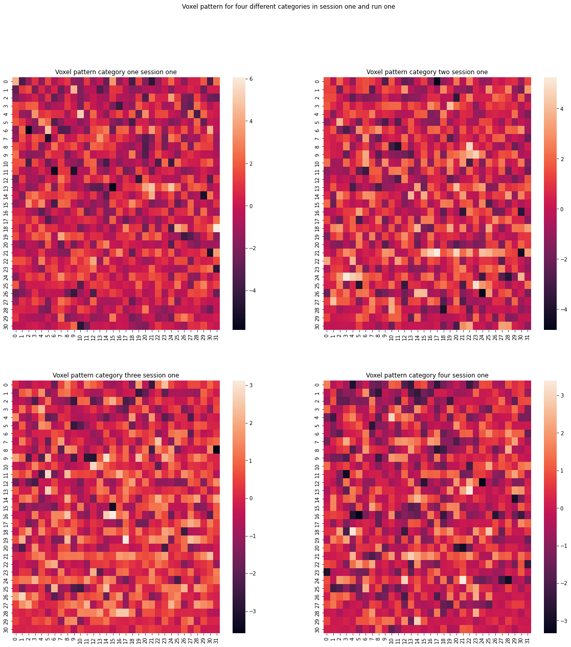
figure.suptitle('Voxel pattern for four different categories in session one and run one')
Text(0.5, 0.98, 'Voxel pattern for four different categories in session one and run one')
figure, axis = plt.subplots(2, 2,figsize=(20, 20))
im1 = sns.heatmap(X_11,ax=axis[0,0])
im2= sns.heatmap(X_21,ax=axis[0,1])
im3= sns.heatmap(X_31,ax=axis[1,0])
im4= sns.heatmap(X_41, ax=axis[1,1])
#figure.colorbar(orientation='vertical')
axis[0, 0].set_title("Voxel pattern category one session two")
axis[0, 1].set_title("Voxel pattern category two session two")
axis[1, 0].set_title("Voxel pattern category three session two")
axis[1, 1].set_title("Voxel pattern category four session two")
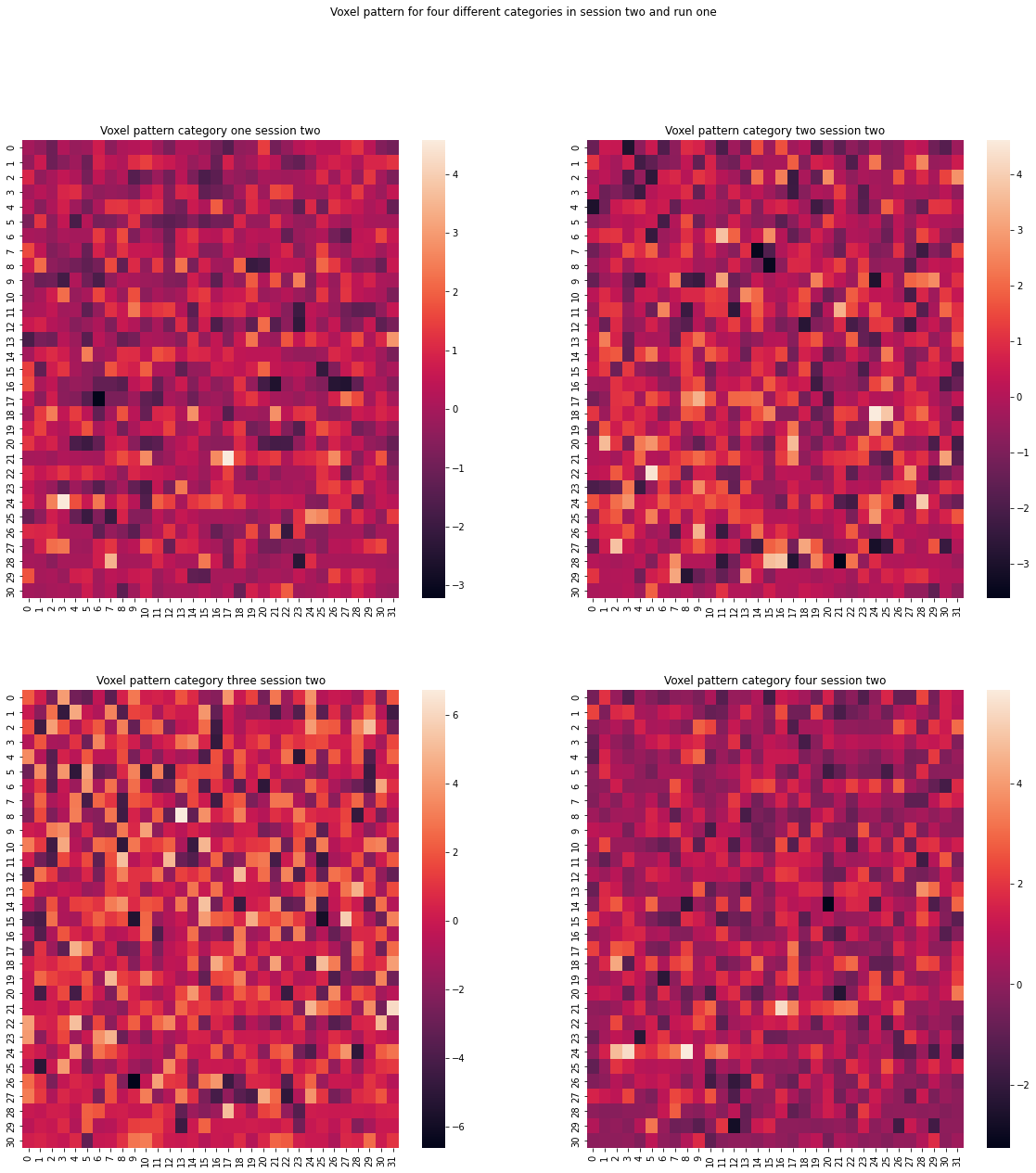
figure.suptitle('Voxel pattern for four different categories in session two and run one')
Text(0.5, 0.98, 'Voxel pattern for four different categories in session two and run one')
figure, axis = plt.subplots(2, 2,figsize=(20, 20))
im1 = sns.heatmap(X_12,ax=axis[0,0])
im2= sns.heatmap(X_22,ax=axis[0,1])
im3= sns.heatmap(X_32,ax=axis[1,0])
im4= sns.heatmap(X_42, ax=axis[1,1])
#figure.colorbar(orientation='vertical')
axis[0, 0].set_title("Voxel pattern category one session three")
axis[0, 1].set_title("Voxel pattern category two session three")
axis[1, 0].set_title("Voxel pattern category three session three")
axis[1, 1].set_title("Voxel pattern category four session three")
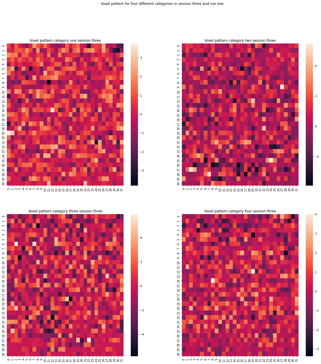
figure.suptitle('Voxel pattern for four different categories in session three and run one')
Text(0.5, 0.98, 'Voxel pattern for four different categories in session three and run one')
figure, axis = plt.subplots(2, 2,figsize=(20, 20))
im1 = sns.heatmap(X_13,ax=axis[0,0])
im2= sns.heatmap(X_23,ax=axis[0,1])
im3= sns.heatmap(X_33,ax=axis[1,0])
im4= sns.heatmap(X_43, ax=axis[1,1])

#figure.colorbar(orientation='vertical')
axis[0, 0].set_title("Voxel pattern category one session four")
axis[0, 1].set_title("Voxel pattern category two session four")
axis[1, 0].set_title("Voxel pattern category three session four")
axis[1, 1].set_title("Voxel pattern category four session four")

figure.suptitle('Voxel pattern for four different categories in session four and run one')
Text(0.5, 0.98, 'Voxel pattern for four different categories in session four and run one')
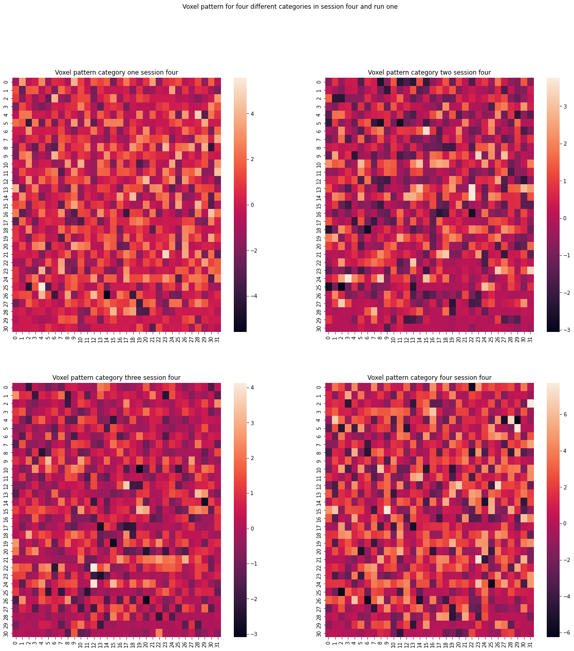
It really seems like there is no clear pattern to be examined between or within sessions. It rather looks like a lot of noise.
3.0 Logistic regression#
This notebook has gone through several attempts. Please take a look at the respective github repository folder to understand the different attempts made.
For example: The first idea was to run the Logistic Regression for the z maps across runs (so 104 samples) with a 80/20 split. This ended up in really bad accuracies. Thus I implemented a GridSearch, to tune the hyperparameters of the model. This did not help. I then tried to create x and y manually. This means, that I created a loop which sorts the data into training and testing set at random, so the model would be trained in instances of all sessions and tested on instances of all sessions. Results remained poorly. Then I tried to run a PCA and inverse transform it without the session variance (please follow this notebook for more detailed explanation). This also did not help. I tried several masks. Nothing. Sklearns feature selection (k-best) did not improve results. I even tried the procedure with the data from subject two. But, you might guess it, nothing changed. Thats why this notebook containts the attempt with using the LOGO strategy and the z-maps perrun. The idea was to increase the samples and let the model “see” more data before testing it.
If you are interested in the other approaches, please take either a look at the open-lab-notebook, the different github versions or contact me.
Otherwise, some of the approaches mentioned are documented in the SVM notebook.
To set up the logistic regression we will mostly use the fantastic machine learning library sklearn.
We will choose the leave one group out method for cross validation. Since we have 4 sessions, we will leave the last session, so session 4, out for testing our data. In the meanwhile, session 1,2 and 3 are cross validated against each other. Meaning, that the logistic regression is trained with the data of session 1 and 2 and then validated against session 3, and so on. This trained model will then be tested on the data from session 4.
But step by step:
Define our group variable, which basically just consists of the respective session label for each sample. This is a neccesary argument for the LeaveOneGroupOut method.
y_ses = np.array(Sessions)
y_ses.shape
(520,)
groups = y_ses[0:390]
groups
array(['1', '1', '1', '1', '1', '1', '1', '1', '1', '1', '1', '1', '1',
       '1', '1', '1', '1', '1', '1', '1', '1', '1', '1', '1', '1', '1',
       '1', '1', '1', '1', '1', '1', '1', '1', '1', '1', '1', '1', '1',
       '1', '1', '1', '1', '1', '1', '1', '1', '1', '1', '1', '1', '1',
       '1', '1', '1', '1', '1', '1', '1', '1', '1', '1', '1', '1', '1',
       '1', '1', '1', '1', '1', '1', '1', '1', '1', '1', '1', '1', '1',
       '1', '1', '1', '1', '1', '1', '1', '1', '1', '1', '1', '1', '1',
       '1', '1', '1', '1', '1', '1', '1', '1', '1', '1', '1', '1', '1',
       '1', '1', '1', '1', '1', '1', '1', '1', '1', '1', '1', '1', '1',
       '1', '1', '1', '1', '1', '1', '1', '1', '1', '1', '1', '1', '1',
       '2', '2', '2', '2', '2', '2', '2', '2', '2', '2', '2', '2', '2',
       '2', '2', '2', '2', '2', '2', '2', '2', '2', '2', '2', '2', '2',
       '2', '2', '2', '2', '2', '2', '2', '2', '2', '2', '2', '2', '2',
       '2', '2', '2', '2', '2', '2', '2', '2', '2', '2', '2', '2', '2',
       '2', '2', '2', '2', '2', '2', '2', '2', '2', '2', '2', '2', '2',
       '2', '2', '2', '2', '2', '2', '2', '2', '2', '2', '2', '2', '2',
       '2', '2', '2', '2', '2', '2', '2', '2', '2', '2', '2', '2', '2',
       '2', '2', '2', '2', '2', '2', '2', '2', '2', '2', '2', '2', '2',
       '2', '2', '2', '2', '2', '2', '2', '2', '2', '2', '2', '2', '2',
       '2', '2', '2', '2', '2', '2', '2', '2', '2', '2', '2', '2', '2',
       '3', '3', '3', '3', '3', '3', '3', '3', '3', '3', '3', '3', '3',
       '3', '3', '3', '3', '3', '3', '3', '3', '3', '3', '3', '3', '3',
       '3', '3', '3', '3', '3', '3', '3', '3', '3', '3', '3', '3', '3',
       '3', '3', '3', '3', '3', '3', '3', '3', '3', '3', '3', '3', '3',
       '3', '3', '3', '3', '3', '3', '3', '3', '3', '3', '3', '3', '3',
       '3', '3', '3', '3', '3', '3', '3', '3', '3', '3', '3', '3', '3',
       '3', '3', '3', '3', '3', '3', '3', '3', '3', '3', '3', '3', '3',
       '3', '3', '3', '3', '3', '3', '3', '3', '3', '3', '3', '3', '3',
       '3', '3', '3', '3', '3', '3', '3', '3', '3', '3', '3', '3', '3',
       '3', '3', '3', '3', '3', '3', '3', '3', '3', '3', '3', '3', '3'],
      dtype='<U1')
The groupsvariable contains the labels for the corresponding sessions.
Split the data in a training testing set. Then, we are also going to normalize our X data with sklearns processing module. In order to do so, we will fit_transform the scaler on to the training data. The scaler has to be solely fitted on to the test data later on.
X_train = X[0:390]
y_train = y[0:390]

X_test = X[390:520] #leaving session 4 out
y_test = y[390:520]
from sklearn import preprocessing
scaler = preprocessing.StandardScaler()
X_train = scaler.fit_transform(X_train)
X_train
array([[ 2.64917891, -2.64553965, -0.99305767, ...,  1.36191438,
         2.75607907, -0.08791735],
       [ 0.77844309,  0.10000231,  1.80385961, ...,  0.17967888,
         0.03273082, -2.62331056],
       [-0.06570151, -0.21416028, -0.56115439, ..., -0.53804601,
        -1.51282094, -0.40462765],
       ...,
       [-1.33283106, -0.63989117,  0.67598363, ...,  0.45854829,
        -0.24723161, -0.67767179],
       [-0.14811615, -0.22006141, -0.01764536, ...,  0.23074111,
        -1.11073331,  0.72772915],
       [-0.4429714 , -0.62463423, -0.64368391, ..., -0.54341624,
         0.75573819,  0.22432805]])
Step one and two are finished. We split our X and y variables into a training and testing set, and normalised our X_train variable.
NOTE: The index for the training and testing set are choosen that way, because the first 390 samples belong to session 1 - 3. Remember: One session has 5 runs per 26 categories. Leaving us with 130 samples per session.
Step 3. Import sklearns LeaveOneGroupOut module. Store the method in a variable ‘LOGO’. Run a loop over our training variables to get an idea, how the method works “behind the scene”:
from sklearn.model_selection import LeaveOneGroupOut

LOGO = LeaveOneGroupOut()
train_i = []
test_i = []
for i, (train_index, test_index) in enumerate(LOGO.split(X_train,y_train,groups)):
    print(f"Fold {i}:")
    print(f"  Train: index={train_index}, group={groups[train_index]}")
    print(f"  Test:  index={test_index}, group={groups[test_index]}")
    train_i.append(train_index)
    test_i.append(test_index)
Fold 0:
  Train: index=[130 131 132 133 134 135 136 137 138 139 140 141 142 143 144 145 146 147
 148 149 150 151 152 153 154 155 156 157 158 159 160 161 162 163 164 165
 166 167 168 169 170 171 172 173 174 175 176 177 178 179 180 181 182 183
 184 185 186 187 188 189 190 191 192 193 194 195 196 197 198 199 200 201
 202 203 204 205 206 207 208 209 210 211 212 213 214 215 216 217 218 219
 220 221 222 223 224 225 226 227 228 229 230 231 232 233 234 235 236 237
 238 239 240 241 242 243 244 245 246 247 248 249 250 251 252 253 254 255
 256 257 258 259 260 261 262 263 264 265 266 267 268 269 270 271 272 273
 274 275 276 277 278 279 280 281 282 283 284 285 286 287 288 289 290 291
 292 293 294 295 296 297 298 299 300 301 302 303 304 305 306 307 308 309
 310 311 312 313 314 315 316 317 318 319 320 321 322 323 324 325 326 327
 328 329 330 331 332 333 334 335 336 337 338 339 340 341 342 343 344 345
 346 347 348 349 350 351 352 353 354 355 356 357 358 359 360 361 362 363
 364 365 366 367 368 369 370 371 372 373 374 375 376 377 378 379 380 381
 382 383 384 385 386 387 388 389], group=['2' '2' '2' '2' '2' '2' '2' '2' '2' '2' '2' '2' '2' '2' '2' '2' '2' '2'
 '2' '2' '2' '2' '2' '2' '2' '2' '2' '2' '2' '2' '2' '2' '2' '2' '2' '2'
 '2' '2' '2' '2' '2' '2' '2' '2' '2' '2' '2' '2' '2' '2' '2' '2' '2' '2'
 '2' '2' '2' '2' '2' '2' '2' '2' '2' '2' '2' '2' '2' '2' '2' '2' '2' '2'
 '2' '2' '2' '2' '2' '2' '2' '2' '2' '2' '2' '2' '2' '2' '2' '2' '2' '2'
 '2' '2' '2' '2' '2' '2' '2' '2' '2' '2' '2' '2' '2' '2' '2' '2' '2' '2'
 '2' '2' '2' '2' '2' '2' '2' '2' '2' '2' '2' '2' '2' '2' '2' '2' '2' '2'
 '2' '2' '2' '2' '3' '3' '3' '3' '3' '3' '3' '3' '3' '3' '3' '3' '3' '3'
 '3' '3' '3' '3' '3' '3' '3' '3' '3' '3' '3' '3' '3' '3' '3' '3' '3' '3'
 '3' '3' '3' '3' '3' '3' '3' '3' '3' '3' '3' '3' '3' '3' '3' '3' '3' '3'
 '3' '3' '3' '3' '3' '3' '3' '3' '3' '3' '3' '3' '3' '3' '3' '3' '3' '3'
 '3' '3' '3' '3' '3' '3' '3' '3' '3' '3' '3' '3' '3' '3' '3' '3' '3' '3'
 '3' '3' '3' '3' '3' '3' '3' '3' '3' '3' '3' '3' '3' '3' '3' '3' '3' '3'
 '3' '3' '3' '3' '3' '3' '3' '3' '3' '3' '3' '3' '3' '3' '3' '3' '3' '3'
 '3' '3' '3' '3' '3' '3' '3' '3']
  Test:  index=[  0   1   2   3   4   5   6   7   8   9  10  11  12  13  14  15  16  17
  18  19  20  21  22  23  24  25  26  27  28  29  30  31  32  33  34  35
  36  37  38  39  40  41  42  43  44  45  46  47  48  49  50  51  52  53
  54  55  56  57  58  59  60  61  62  63  64  65  66  67  68  69  70  71
  72  73  74  75  76  77  78  79  80  81  82  83  84  85  86  87  88  89
  90  91  92  93  94  95  96  97  98  99 100 101 102 103 104 105 106 107
 108 109 110 111 112 113 114 115 116 117 118 119 120 121 122 123 124 125
 126 127 128 129], group=['1' '1' '1' '1' '1' '1' '1' '1' '1' '1' '1' '1' '1' '1' '1' '1' '1' '1'
 '1' '1' '1' '1' '1' '1' '1' '1' '1' '1' '1' '1' '1' '1' '1' '1' '1' '1'
 '1' '1' '1' '1' '1' '1' '1' '1' '1' '1' '1' '1' '1' '1' '1' '1' '1' '1'
 '1' '1' '1' '1' '1' '1' '1' '1' '1' '1' '1' '1' '1' '1' '1' '1' '1' '1'
 '1' '1' '1' '1' '1' '1' '1' '1' '1' '1' '1' '1' '1' '1' '1' '1' '1' '1'
 '1' '1' '1' '1' '1' '1' '1' '1' '1' '1' '1' '1' '1' '1' '1' '1' '1' '1'
 '1' '1' '1' '1' '1' '1' '1' '1' '1' '1' '1' '1' '1' '1' '1' '1' '1' '1'
 '1' '1' '1' '1']
Fold 1:
  Train: index=[  0   1   2   3   4   5   6   7   8   9  10  11  12  13  14  15  16  17
  18  19  20  21  22  23  24  25  26  27  28  29  30  31  32  33  34  35
  36  37  38  39  40  41  42  43  44  45  46  47  48  49  50  51  52  53
  54  55  56  57  58  59  60  61  62  63  64  65  66  67  68  69  70  71
  72  73  74  75  76  77  78  79  80  81  82  83  84  85  86  87  88  89
  90  91  92  93  94  95  96  97  98  99 100 101 102 103 104 105 106 107
 108 109 110 111 112 113 114 115 116 117 118 119 120 121 122 123 124 125
 126 127 128 129 260 261 262 263 264 265 266 267 268 269 270 271 272 273
 274 275 276 277 278 279 280 281 282 283 284 285 286 287 288 289 290 291
 292 293 294 295 296 297 298 299 300 301 302 303 304 305 306 307 308 309
 310 311 312 313 314 315 316 317 318 319 320 321 322 323 324 325 326 327
 328 329 330 331 332 333 334 335 336 337 338 339 340 341 342 343 344 345
 346 347 348 349 350 351 352 353 354 355 356 357 358 359 360 361 362 363
 364 365 366 367 368 369 370 371 372 373 374 375 376 377 378 379 380 381
 382 383 384 385 386 387 388 389], group=['1' '1' '1' '1' '1' '1' '1' '1' '1' '1' '1' '1' '1' '1' '1' '1' '1' '1'
 '1' '1' '1' '1' '1' '1' '1' '1' '1' '1' '1' '1' '1' '1' '1' '1' '1' '1'
 '1' '1' '1' '1' '1' '1' '1' '1' '1' '1' '1' '1' '1' '1' '1' '1' '1' '1'
 '1' '1' '1' '1' '1' '1' '1' '1' '1' '1' '1' '1' '1' '1' '1' '1' '1' '1'
 '1' '1' '1' '1' '1' '1' '1' '1' '1' '1' '1' '1' '1' '1' '1' '1' '1' '1'
 '1' '1' '1' '1' '1' '1' '1' '1' '1' '1' '1' '1' '1' '1' '1' '1' '1' '1'
 '1' '1' '1' '1' '1' '1' '1' '1' '1' '1' '1' '1' '1' '1' '1' '1' '1' '1'
 '1' '1' '1' '1' '3' '3' '3' '3' '3' '3' '3' '3' '3' '3' '3' '3' '3' '3'
 '3' '3' '3' '3' '3' '3' '3' '3' '3' '3' '3' '3' '3' '3' '3' '3' '3' '3'
 '3' '3' '3' '3' '3' '3' '3' '3' '3' '3' '3' '3' '3' '3' '3' '3' '3' '3'
 '3' '3' '3' '3' '3' '3' '3' '3' '3' '3' '3' '3' '3' '3' '3' '3' '3' '3'
 '3' '3' '3' '3' '3' '3' '3' '3' '3' '3' '3' '3' '3' '3' '3' '3' '3' '3'
 '3' '3' '3' '3' '3' '3' '3' '3' '3' '3' '3' '3' '3' '3' '3' '3' '3' '3'
 '3' '3' '3' '3' '3' '3' '3' '3' '3' '3' '3' '3' '3' '3' '3' '3' '3' '3'
 '3' '3' '3' '3' '3' '3' '3' '3']
  Test:  index=[130 131 132 133 134 135 136 137 138 139 140 141 142 143 144 145 146 147
 148 149 150 151 152 153 154 155 156 157 158 159 160 161 162 163 164 165
 166 167 168 169 170 171 172 173 174 175 176 177 178 179 180 181 182 183
 184 185 186 187 188 189 190 191 192 193 194 195 196 197 198 199 200 201
 202 203 204 205 206 207 208 209 210 211 212 213 214 215 216 217 218 219
 220 221 222 223 224 225 226 227 228 229 230 231 232 233 234 235 236 237
 238 239 240 241 242 243 244 245 246 247 248 249 250 251 252 253 254 255
 256 257 258 259], group=['2' '2' '2' '2' '2' '2' '2' '2' '2' '2' '2' '2' '2' '2' '2' '2' '2' '2'
 '2' '2' '2' '2' '2' '2' '2' '2' '2' '2' '2' '2' '2' '2' '2' '2' '2' '2'
 '2' '2' '2' '2' '2' '2' '2' '2' '2' '2' '2' '2' '2' '2' '2' '2' '2' '2'
 '2' '2' '2' '2' '2' '2' '2' '2' '2' '2' '2' '2' '2' '2' '2' '2' '2' '2'
 '2' '2' '2' '2' '2' '2' '2' '2' '2' '2' '2' '2' '2' '2' '2' '2' '2' '2'
 '2' '2' '2' '2' '2' '2' '2' '2' '2' '2' '2' '2' '2' '2' '2' '2' '2' '2'
 '2' '2' '2' '2' '2' '2' '2' '2' '2' '2' '2' '2' '2' '2' '2' '2' '2' '2'
 '2' '2' '2' '2']
Fold 2:
  Train: index=[  0   1   2   3   4   5   6   7   8   9  10  11  12  13  14  15  16  17
  18  19  20  21  22  23  24  25  26  27  28  29  30  31  32  33  34  35
  36  37  38  39  40  41  42  43  44  45  46  47  48  49  50  51  52  53
  54  55  56  57  58  59  60  61  62  63  64  65  66  67  68  69  70  71
  72  73  74  75  76  77  78  79  80  81  82  83  84  85  86  87  88  89
  90  91  92  93  94  95  96  97  98  99 100 101 102 103 104 105 106 107
 108 109 110 111 112 113 114 115 116 117 118 119 120 121 122 123 124 125
 126 127 128 129 130 131 132 133 134 135 136 137 138 139 140 141 142 143
 144 145 146 147 148 149 150 151 152 153 154 155 156 157 158 159 160 161
 162 163 164 165 166 167 168 169 170 171 172 173 174 175 176 177 178 179
 180 181 182 183 184 185 186 187 188 189 190 191 192 193 194 195 196 197
 198 199 200 201 202 203 204 205 206 207 208 209 210 211 212 213 214 215
 216 217 218 219 220 221 222 223 224 225 226 227 228 229 230 231 232 233
 234 235 236 237 238 239 240 241 242 243 244 245 246 247 248 249 250 251
 252 253 254 255 256 257 258 259], group=['1' '1' '1' '1' '1' '1' '1' '1' '1' '1' '1' '1' '1' '1' '1' '1' '1' '1'
 '1' '1' '1' '1' '1' '1' '1' '1' '1' '1' '1' '1' '1' '1' '1' '1' '1' '1'
 '1' '1' '1' '1' '1' '1' '1' '1' '1' '1' '1' '1' '1' '1' '1' '1' '1' '1'
 '1' '1' '1' '1' '1' '1' '1' '1' '1' '1' '1' '1' '1' '1' '1' '1' '1' '1'
 '1' '1' '1' '1' '1' '1' '1' '1' '1' '1' '1' '1' '1' '1' '1' '1' '1' '1'
 '1' '1' '1' '1' '1' '1' '1' '1' '1' '1' '1' '1' '1' '1' '1' '1' '1' '1'
 '1' '1' '1' '1' '1' '1' '1' '1' '1' '1' '1' '1' '1' '1' '1' '1' '1' '1'
 '1' '1' '1' '1' '2' '2' '2' '2' '2' '2' '2' '2' '2' '2' '2' '2' '2' '2'
 '2' '2' '2' '2' '2' '2' '2' '2' '2' '2' '2' '2' '2' '2' '2' '2' '2' '2'
 '2' '2' '2' '2' '2' '2' '2' '2' '2' '2' '2' '2' '2' '2' '2' '2' '2' '2'
 '2' '2' '2' '2' '2' '2' '2' '2' '2' '2' '2' '2' '2' '2' '2' '2' '2' '2'
 '2' '2' '2' '2' '2' '2' '2' '2' '2' '2' '2' '2' '2' '2' '2' '2' '2' '2'
 '2' '2' '2' '2' '2' '2' '2' '2' '2' '2' '2' '2' '2' '2' '2' '2' '2' '2'
 '2' '2' '2' '2' '2' '2' '2' '2' '2' '2' '2' '2' '2' '2' '2' '2' '2' '2'
 '2' '2' '2' '2' '2' '2' '2' '2']
  Test:  index=[260 261 262 263 264 265 266 267 268 269 270 271 272 273 274 275 276 277
 278 279 280 281 282 283 284 285 286 287 288 289 290 291 292 293 294 295
 296 297 298 299 300 301 302 303 304 305 306 307 308 309 310 311 312 313
 314 315 316 317 318 319 320 321 322 323 324 325 326 327 328 329 330 331
 332 333 334 335 336 337 338 339 340 341 342 343 344 345 346 347 348 349
 350 351 352 353 354 355 356 357 358 359 360 361 362 363 364 365 366 367
 368 369 370 371 372 373 374 375 376 377 378 379 380 381 382 383 384 385
 386 387 388 389], group=['3' '3' '3' '3' '3' '3' '3' '3' '3' '3' '3' '3' '3' '3' '3' '3' '3' '3'
 '3' '3' '3' '3' '3' '3' '3' '3' '3' '3' '3' '3' '3' '3' '3' '3' '3' '3'
 '3' '3' '3' '3' '3' '3' '3' '3' '3' '3' '3' '3' '3' '3' '3' '3' '3' '3'
 '3' '3' '3' '3' '3' '3' '3' '3' '3' '3' '3' '3' '3' '3' '3' '3' '3' '3'
 '3' '3' '3' '3' '3' '3' '3' '3' '3' '3' '3' '3' '3' '3' '3' '3' '3' '3'
 '3' '3' '3' '3' '3' '3' '3' '3' '3' '3' '3' '3' '3' '3' '3' '3' '3' '3'
 '3' '3' '3' '3' '3' '3' '3' '3' '3' '3' '3' '3' '3' '3' '3' '3' '3' '3'
 '3' '3' '3' '3']
We now have an idea of how the LOGO method works. it is time to setup our Logistic Regression model. We will define and then fit it on the training data. Afterwards, we will take a look on how well it can predict the test data.
For this part we need sklearns LogisticRegression function. This method allows us to set up the one versus rest(ovr) multi_class classification algorithm. OVR allows us to compare one class (for example image category one) vs all the other classes (category 2-25). So one model is created for each class. Each model predicts a probability for a given class. The highest probability is then used as a predictor.
cv=LeaveOneGroupOut().split(X_train, y_train, groups)
from sklearn.linear_model import LogisticRegression
model = LogisticRegression(C=1,multi_class='ovr', penalty = 'l1', solver = 'liblinear')
from sklearn.model_selection import cross_val_score
cross_val_score(model,X_train,y_train,cv=cv)
array([0.02307692, 0.03846154, 0.03846154])
So those cross validation scores, generated by using sklearns ‘cross_val_score’ method gives us three accuracy scores. Each score represents how well the model could predict the labels based on the LOGO method. So score # 1 is how well the model predicts the labels in session one, when trained on session two and three. Score # 2 based on training the data with session one and three and testing on two, and Score # 3 training the data with session one and two and tested on session three.
Overall the scores are…. very bad, meaning very inaccurate. Accuracy is defined as the fraction of correct predicted labels. This basically means, our model could not predict anything at all. Yikes. We will proceed anyway by fitting a LogisticRegression on the training data (still using our LOGO cross validation) and then testing it on session 4.
from sklearn.linear_model import LogisticRegressionCV
cv=LeaveOneGroupOut().split(X_train, y_train, groups)
LOGOReg= LogisticRegressionCV(multi_class='ovr', penalty = 'l2', solver = 'liblinear',cv=cv)
LOGOReg.fit(X_train,y_train)
LogisticRegressionCV(cv=<generator object BaseCrossValidator.split at 0x7fda08e72ed0>,
                     multi_class='ovr', solver='liblinear')
LOGOReg.score(X_train,y_train)
1.0
LOGOReg.score(scaler.transform(X_test),y_test)
0.06153846153846154
After fitting our model is becomes very obvious, that we could not predict anything at all in the testing data. Our model seems to be dramatically overfitted.
But lets visualize our results. We can create a classification_report and a confusion matrix.
from sklearn.metrics import classification_report
y_train_pred = LOGOReg.predict(X_train)
print(classification_report(y_train, y_train_pred))
              precision    recall  f1-score   support

           1       1.00      1.00      1.00        15
           2       1.00      1.00      1.00        15
           3       1.00      1.00      1.00        15
           4       1.00      1.00      1.00        15
           5       1.00      1.00      1.00        15
           6       1.00      1.00      1.00        15
           7       1.00      1.00      1.00        15
           8       1.00      1.00      1.00        15
           9       1.00      1.00      1.00        15
          10       1.00      1.00      1.00        15
          11       1.00      1.00      1.00        15
          12       1.00      1.00      1.00        15
          13       1.00      1.00      1.00        15
          14       1.00      1.00      1.00        15
          15       1.00      1.00      1.00        15
          16       1.00      1.00      1.00        15
          17       1.00      1.00      1.00        15
          18       1.00      1.00      1.00        15
          19       1.00      1.00      1.00        15
          20       1.00      1.00      1.00        15
          21       1.00      1.00      1.00        15
          22       1.00      1.00      1.00        15
          23       1.00      1.00      1.00        15
          24       1.00      1.00      1.00        15
          25       1.00      1.00      1.00        15
          26       1.00      1.00      1.00        15

    accuracy                           1.00       390
   macro avg       1.00      1.00      1.00       390
weighted avg       1.00      1.00      1.00       390
y_test_pred = LOGOReg.predict(X_test)
print(classification_report(y_test, y_test_pred))
              precision    recall  f1-score   support

           1       0.00      0.00      0.00         5
           2       0.00      0.00      0.00         5
           3       0.00      0.00      0.00         5
           4       0.00      0.00      0.00         5
           5       0.00      0.00      0.00         5
           6       0.00      0.00      0.00         5
           7       0.00      0.00      0.00         5
           8       0.00      0.00      0.00         5
           9       0.00      0.00      0.00         5
          10       0.00      0.00      0.00         5
          11       0.00      0.00      0.00         5
          12       0.20      0.20      0.20         5
          13       0.06      0.60      0.11         5
          14       0.00      0.00      0.00         5
          15       0.00      0.00      0.00         5
          16       0.00      0.00      0.00         5
          17       0.00      0.00      0.00         5
          18       0.00      0.00      0.00         5
          19       0.00      0.00      0.00         5
          20       0.50      0.20      0.29         5
          21       0.00      0.00      0.00         5
          22       0.00      0.00      0.00         5
          23       0.00      0.00      0.00         5
          24       0.33      0.20      0.25         5
          25       0.00      0.00      0.00         5
          26       0.00      0.00      0.00         5

    accuracy                           0.05       130
   macro avg       0.04      0.05      0.03       130
weighted avg       0.04      0.05      0.03       130
/home/jpauli/miniconda3/envs/neuro_ai/lib/python3.7/site-packages/sklearn/metrics/_classification.py:1318: UndefinedMetricWarning: Precision and F-score are ill-defined and being set to 0.0 in labels with no predicted samples. Use `zero_division` parameter to control this behavior.
  _warn_prf(average, modifier, msg_start, len(result))
Explaination:
Precision is the ratio of true positives (tp) / (tp + false positives (fp))
Recall is the ratio of tp / (tp + false negatives (fn))
“The F-beta score can be interpreted as a weighted harmonic mean of the precision and recall, where an F-beta score reaches its best value at 1 and worst score at 0.”
Support refers to the occurrences of the respective class in y_true.
Source: Sklearn documentation
The classification reports tell us that the training data is 100% predicted and the test data 0% predicted.
from sklearn.metrics import confusion_matrix
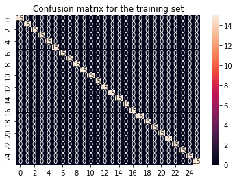
cf_matrix_train = confusion_matrix(y_train, y_train_pred)
sns.heatmap(cf_matrix_train, annot = True).set(title='Confusion matrix for the training set');
cf_matrix_test = confusion_matrix(y_test, y_test_pred)
sns.heatmap(cf_matrix_test, annot = True).set(title='Confusion matrix for the testing set');
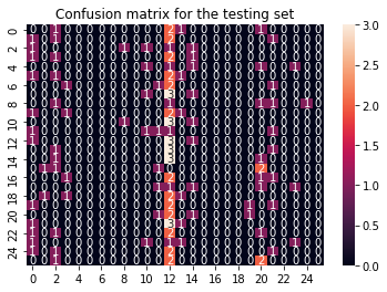
This does not look too good. Apparently our training data can be predicted very well, but on the test data the algorithm performs very poor. This is illustrated clearly in the confusion matrix. Well organized for the train confusion matrix but just a mess in the test confusion matrix.
4.0 Error search - what is wrong with the data?#
Since the model did not perform well at all, we should inspect what exactly is going wrong. For example, we have a lot of features (992) but only 520 samples. This combination is prone to overfitting. Thus, we should continue with examining the feature importance. Meaning, inspecting which features are actually important for the model and which are not.
Each feature gets a certain weight assigned by the Logistic Regression. This loop goes through all those coefficients. We will go through all weights, that are at least above 1.0 and plot them. The weight determines, how important the feature is.
coef = LOGOReg.coef_
imp_f = []
imp_coef = []
j= 0

while j < 26:
    for feature, coefficient in enumerate(coef[j]):
        if coefficient > 1 or coefficient < -1:
            imp_f.append(feature)
            imp_coef.append(coefficient)
    j=j+1
import matplotlib.pyplot as plt
plt.plot(coef[0])
plt.plot(coef[1])
plt.plot(coef[2])
plt.plot(coef[3])
plt.title('Coefficients for category one, two, three and four');
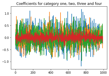
Not a lot of cofficients seem to be above 0.5. That doesnt look good. Rather that there are a lot of non meaningful coefficients.
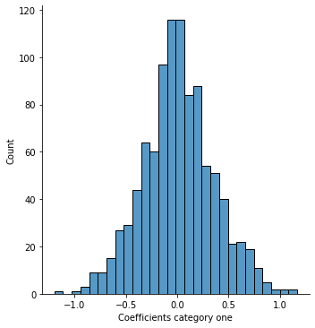
We continue with plotting the coefficients for category one and two
sns.displot(coef[0])
plt.xlabel('Coefficients category one');
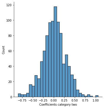
sns.displot(coef[1])
plt.xlabel('Coefficients category two');
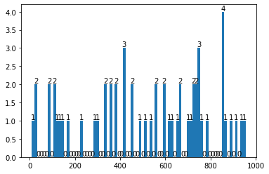
We can now plot all important features (so features that have a weight greater than 0.5) in a bar plot, to get an idea, which features might be more important than others. Also, we can choose those features and run our logistic regression model again.
print('There seem to be {} features that are <important>'.format(len(imp_f)))
There seem to be 57 features that are <important>
counts, edges, bars = plt.hist(imp_f,density=False, bins = 80)
plt.bar_label(bars);
print(counts)
[1. 2. 0. 0. 0. 0. 2. 0. 2. 1. 1. 1. 0. 1. 0. 0. 0. 0. 1. 0. 0. 0. 0. 1.
 1. 0. 0. 2. 0. 2. 0. 2. 0. 0. 3. 0. 0. 2. 0. 0. 1. 0. 1. 0. 1. 0. 2. 0.
 0. 2. 0. 1. 1. 0. 1. 2. 0. 0. 1. 1. 2. 2. 3. 1. 0. 1. 0. 0. 0. 0. 0. 4.
 1. 0. 1. 0. 1. 0. 1. 1.]
We get all unique features from the important features list to use them as our input features.
unique_features = np.unique(imp_f)
unique_features.shape
(56,)
X_imp = X[:,[unique_features]]
X_imp.shape
X_imp = np.reshape(X_imp, (520,56))
X_imp.shape
(520, 56)
X_imp now represents our input data, but with 936 features (=voxel) less. This might be an idea to combat overfitting.
The remaining 56 features are somewhat important. So lets run the logistic regression again!
To prevent myself from repeating information, I will not provide a lot of information here. All steps from above are repeated.
X_imp_train = X_imp[0:390]
X_imp_test = X_imp[390:520]
X_imp_train = scaler.fit_transform(X_imp_train)
cv=LeaveOneGroupOut().split(X_imp_train, y_train, groups)
LogRegimp = LogisticRegressionCV(multi_class = 'ovr', penalty = 'l1', solver = 'liblinear', cv = cv)
LogRegimp.fit(X_imp_train,y_train)
LogisticRegressionCV(cv=<generator object BaseCrossValidator.split at 0x7fda06d3a570>,
                     multi_class='ovr', penalty='l1', solver='liblinear')
LogRegimp.score(X_imp_train,y_train)
0.038461538461538464
LogRegimp.score(scaler.transform(X_imp_test),y_test)
0.038461538461538464
y_pred_train = LogRegimp.predict(X_imp_train)
cf_matrix_train = confusion_matrix(y_train, y_pred_train)
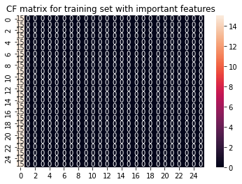
sns.heatmap(cf_matrix_train, annot = True).set(title='CF matrix for training set with important features');
y_pred = LogRegimp.predict(scaler.transform(X_imp_test))
cf_matrix = confusion_matrix(y_test, y_pred)
sns.heatmap(cf_matrix, annot=True).set(title='CF matrix for testing set with important features');
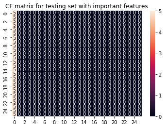
To sum this section up: Our model does not work. Feature selection does not help. SklearnsGridSearch also does not help. Manually adjusting the y labels does not help either. Running the glm per run to get more samples does not work. Cross validation does not work… You’ll get the idea.
To proceed, we will now fit a PCA onto the data. Most likely, the high within session correlation is at fault for those poor results.
4.1 PCA#
from sklearn.decomposition import PCA
pca = PCA() #n_components = 10
pca.fit(X)
PCA()
plt.plot(pca.explained_variance_ratio_)
[<matplotlib.lines.Line2D at 0x7fda05c37b70>]
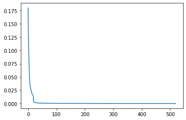
It seems like there are around 20 components, that account for most of the explained variance. We will now transform and then plot the transformed X array.
X_transform = pca.transform(X)
X_transform.shape
(520, 520)
corr =np.corrcoef(X_transform)
plt.matshow(corr, cmap='coolwarm')
plt.colorbar()
plt.xlabel('Samples')
plt.ylabel('Samples')
Text(0, 0.5, 'Samples')
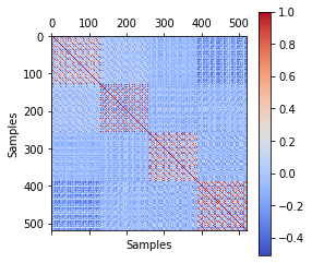
Once again, this shows us the very high correlation within sessions.
We can now create a gaussian noise array, that has the same shape as our input variable X, and plot it together with the explained variance ratio of the original PCA.
rand_X = np.random.normal(size=X.shape)
pca_rand = PCA()
pca_rand.fit(rand_X)
PCA()
plt.plot(pca.explained_variance_ratio_[:25])
plt.plot(pca_rand.explained_variance_ratio_[:25])
[<matplotlib.lines.Line2D at 0x7fda0663a240>]
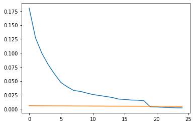
Most of the variance seems to be within 20 components. We have 4 sessions a 5 runs. Meaning, that most of the variance is stuck within those sessions. Everything beyond that is just noise. Our data has a very high within session variance. Making it almost impossible to model anything. For the correlation matrix, we should expect 26 correlation cluster and not only 4. Our model and hypothesis will thus not work. We are unable to dedocde anything beyond noise.
Still, we will continue our journey of diving into the science of computational neuroscience. The next sections will test the same hypothesis with a SVM and a fully conncected neural network.