Dataset Exploration#
0. Introduction#
Explorationof the dataset used in my research project.
This notebook serves the purpose of exploring the structure of the dataset. More precisely, there are two parts within this notebook. The first part will explore the BIDS format. This is done by using the pybids module. The second part will focus on exploring the anatomical and functional files for subject one, within the first session and first run. Next to files of anatomical and functional nature, the events and bold.json files of the respective subject are investigated.
Within the study of the respective dataset, the participants had two main tasks that are interesting for us in the fMRI. Task one was to simply look at visual stimuli (natural images, artifical shapes and alphabetical letters). Task two was to perform mental imagery, so visually imagine one of the presented stimuli. The imagination has been performed on either the natural images or the alphabetical letters.
Example task#
In the paradigm, two experiments were used. To make the paradigm more clear, I will provide a brief example on how a task in the visual stimuli and in the imagery experiment looks like.
Visual stimuli
For the visual stimuli, or image presentation, experiment there were four distinct sessions. 1: Training of the natural images, 2. test of the natural images, artificial shape session and alphabetic letter sessions. For these sessions, each run compromised of 50, 50, 40 and 10 blocks with different images. Since we are mainly interested in the mental imagery part of the experiment, we will now introduce more thoroughly this respective condition. So the main stimuli were natural images, artificial shapes and alphabetic letters.
Mental imagery
As mentioned before, the subject had to recall one of the 25 visual stimuli from the natural images (10) and artificial shape session (15). The visual stimuli were related to a certain word, that helps them with the recall by using a word-cue. The imagery part consisted of 20 seperate runs, each run with 26 blocks. The 26 blocks were built from 25 imagery trials and one fixation trial. In the fixation trial no imagery was performed.
The imagery trials looked like this: 4 seconds of word-cue, 8 seconds of imagery, 3 seconds of evalution (how vivid was the imagination) and one second rest period. In the word-cue period, the respective words to indicate the visual stimuli were presented. The participants had to immediately perform the imagery after receiving the word-cue.
1. Exploration of the dataset with pybids#
Bids Validation#
According to the BIDS validator from Openneuro.org the dataset follows a valid BIDS.
We want to understand the structure of the dataset, especially how the dataset follows the BIDS format. This can be done with the pybids module. The following part serves the purpose of determining the structure. To explore the dataset, we will need to obtain it first from datalad. The installation of the dataset is done by using the command datalad install https: OpenNeuroDatasets/ds001506.git in bash.
datalad install OpenNeuroDatasets/ds001506.git
Now we will create a path to where the data is stored and import all modules we need for know. This dataset_path can then be used to investigate the layout of the dataset.
dataset_path = '/home/jpauli/ds001506'
from bids import BIDSLayout
from bids.tests import get_test_data_path
import os
layout = BIDSLayout(dataset_path)
layout
BIDS Layout: .../home/jpauli/ds001506 | Subjects: 3 | Sessions: 77 | Runs: 36
layout.get_tasks()
['imagery', 'perception']
Also, it is possible to get the files of the subjects filtered by the task.
layout.get(subject='01', return_type='file', task="perception")[:10]
['/home/jpauli/ds001506/sub-01/ses-perceptionArtificialImage01/func/sub-01_ses-perceptionArtificialImage01_task-perception_run-01_bold.json',
 '/home/jpauli/ds001506/sub-01/ses-perceptionArtificialImage01/func/sub-01_ses-perceptionArtificialImage01_task-perception_run-01_bold.nii.gz',
 '/home/jpauli/ds001506/sub-01/ses-perceptionArtificialImage01/func/sub-01_ses-perceptionArtificialImage01_task-perception_run-01_events.tsv',
 '/home/jpauli/ds001506/sub-01/ses-perceptionArtificialImage01/func/sub-01_ses-perceptionArtificialImage01_task-perception_run-02_bold.json',
 '/home/jpauli/ds001506/sub-01/ses-perceptionArtificialImage01/func/sub-01_ses-perceptionArtificialImage01_task-perception_run-02_bold.nii.gz',
 '/home/jpauli/ds001506/sub-01/ses-perceptionArtificialImage01/func/sub-01_ses-perceptionArtificialImage01_task-perception_run-02_events.tsv',
 '/home/jpauli/ds001506/sub-01/ses-perceptionArtificialImage01/func/sub-01_ses-perceptionArtificialImage01_task-perception_run-03_bold.json',
 '/home/jpauli/ds001506/sub-01/ses-perceptionArtificialImage01/func/sub-01_ses-perceptionArtificialImage01_task-perception_run-03_bold.nii.gz',
 '/home/jpauli/ds001506/sub-01/ses-perceptionArtificialImage01/func/sub-01_ses-perceptionArtificialImage01_task-perception_run-03_events.tsv',
 '/home/jpauli/ds001506/sub-01/ses-perceptionArtificialImage01/func/sub-01_ses-perceptionArtificialImage01_task-perception_run-04_bold.json']
Also we see, that this is according to BIDS.
layout.get(subject='01', return_type='file', task="imagery")[:10]
['/home/jpauli/ds001506/sub-01/ses-imagery01/func/sub-01_ses-imagery01_task-imagery_run-01_bold.json',
 '/home/jpauli/ds001506/sub-01/ses-imagery01/func/sub-01_ses-imagery01_task-imagery_run-01_bold.nii.gz',
 '/home/jpauli/ds001506/sub-01/ses-imagery01/func/sub-01_ses-imagery01_task-imagery_run-01_events.tsv',
 '/home/jpauli/ds001506/sub-01/ses-imagery01/func/sub-01_ses-imagery01_task-imagery_run-02_bold.json',
 '/home/jpauli/ds001506/sub-01/ses-imagery01/func/sub-01_ses-imagery01_task-imagery_run-02_bold.nii.gz',
 '/home/jpauli/ds001506/sub-01/ses-imagery01/func/sub-01_ses-imagery01_task-imagery_run-02_events.tsv',
 '/home/jpauli/ds001506/sub-01/ses-imagery01/func/sub-01_ses-imagery01_task-imagery_run-03_bold.json',
 '/home/jpauli/ds001506/sub-01/ses-imagery01/func/sub-01_ses-imagery01_task-imagery_run-03_bold.nii.gz',
 '/home/jpauli/ds001506/sub-01/ses-imagery01/func/sub-01_ses-imagery01_task-imagery_run-03_events.tsv',
 '/home/jpauli/ds001506/sub-01/ses-imagery01/func/sub-01_ses-imagery01_task-imagery_run-04_bold.json']
..this is also true for the imagery task!
We can use the following command to get all entitites (=BIDS defined keywords) for our dataset.
layout.get_entities()
{'subject': <Entity subject (pattern=[/\\]+sub-([a-zA-Z0-9]+), dtype=<class 'str'>)>,
 'session': <Entity session (pattern=[_/\\]+ses-([a-zA-Z0-9]+), dtype=<class 'str'>)>,
 'sample': <Entity sample (pattern=[_/\\]+sample-([a-zA-Z0-9]+), dtype=<class 'str'>)>,
 'task': <Entity task (pattern=[_/\\]+task-([a-zA-Z0-9]+), dtype=<class 'str'>)>,
 'acquisition': <Entity acquisition (pattern=[_/\\]+acq-([a-zA-Z0-9]+), dtype=<class 'str'>)>,
 'ceagent': <Entity ceagent (pattern=[_/\\]+ce-([a-zA-Z0-9]+), dtype=<class 'str'>)>,
 'staining': <Entity staining (pattern=[_/\\]+stain-([a-zA-Z0-9]+), dtype=<class 'str'>)>,
 'tracer': <Entity tracer (pattern=[_/\\]+trc-([a-zA-Z0-9]+), dtype=<class 'str'>)>,
 'reconstruction': <Entity reconstruction (pattern=[_/\\]+rec-([a-zA-Z0-9]+), dtype=<class 'str'>)>,
 'direction': <Entity direction (pattern=[_/\\]+dir-([a-zA-Z0-9]+), dtype=<class 'str'>)>,
 'run': <Entity run (pattern=[_/\\]+run-(\d+), dtype=<class 'bids.layout.utils.PaddedInt'>)>,
 'proc': <Entity proc (pattern=[_/\\]+proc-([a-zA-Z0-9]+), dtype=<class 'str'>)>,
 'modality': <Entity modality (pattern=[_/\\]+mod-([a-zA-Z0-9]+), dtype=<class 'str'>)>,
 'echo': <Entity echo (pattern=[_/\\]+echo-([0-9]+), dtype=<class 'str'>)>,
 'flip': <Entity flip (pattern=[_/\\]+flip-([0-9]+), dtype=<class 'str'>)>,
 'inv': <Entity inv (pattern=[_/\\]+inv-([0-9]+), dtype=<class 'str'>)>,
 'mt': <Entity mt (pattern=[_/\\]+mt-(on|off), dtype=<class 'str'>)>,
 'part': <Entity part (pattern=[_/\\]+part-(imag|mag|phase|real), dtype=<class 'str'>)>,
 'recording': <Entity recording (pattern=[_/\\]+recording-([a-zA-Z0-9]+), dtype=<class 'str'>)>,
 'space': <Entity space (pattern=[_/\\]+space-([a-zA-Z0-9]+), dtype=<class 'str'>)>,
 'chunk': <Entity chunk (pattern=[_/\\]+chunk-([0-9]+), dtype=<class 'str'>)>,
 'suffix': <Entity suffix (pattern=[._]*([a-zA-Z0-9]*?)\.[^/\\]+$, dtype=<class 'str'>)>,
 'scans': <Entity scans (pattern=(.*\_scans.tsv)$, dtype=<class 'str'>)>,
 'fmap': <Entity fmap (pattern=(phasediff|magnitude[1-2]|phase[1-2]|fieldmap|epi)\.nii, dtype=<class 'str'>)>,
 'datatype': <Entity datatype (pattern=[/\\]+(anat|beh|dwi|eeg|fmap|func|ieeg|meg|micr|perf|pet)[/\\]+, dtype=<class 'str'>)>,
 'extension': <Entity extension (pattern=[._]*[a-zA-Z0-9]*?(\.[^/\\]+)$, dtype=<class 'str'>)>,
 'Manufacturer': <Entity Manufacturer (pattern=None, dtype=<class 'str'>)>,
 'ManufacturersModelName': <Entity ManufacturersModelName (pattern=None, dtype=<class 'str'>)>,
 'MagneticFieldStrength': <Entity MagneticFieldStrength (pattern=None, dtype=<class 'str'>)>,
 'FlipAngle': <Entity FlipAngle (pattern=None, dtype=<class 'str'>)>,
 'EchoTime': <Entity EchoTime (pattern=None, dtype=<class 'str'>)>,
 'RepetitionTime': <Entity RepetitionTime (pattern=None, dtype=<class 'str'>)>,
 'SliceTiming': <Entity SliceTiming (pattern=None, dtype=<class 'str'>)>,
 'MultibandAccelerationFactor': <Entity MultibandAccelerationFactor (pattern=None, dtype=<class 'str'>)>,
 'TaskName': <Entity TaskName (pattern=None, dtype=<class 'str'>)>}
Lets explore the file of subject 01 a bit more. We can assing the variable “sub1” to the fourth file of subject one, print it out and check the type of the file. This type can then be compared to the intial layout file!
sub1 = layout.get(subject=['01'])[3]
sub1
<BIDSImageFile filename='/home/jpauli/ds001506/sub-01/ses-imagery01/func/sub-01_ses-imagery01_task-imagery_run-01_bold.nii.gz'>
print("The type of this file is:")
type(sub1)
The type of this file is:
bids.layout.models.BIDSImageFile
print("The type of the intial layout file is:")
type(layout)
The type of the intial layout file is:
bids.layout.layout.BIDSLayout
We can now print the metadata associated with this particular file. This metadata is simply the associated .json file. We get information about the magnetic field or the repetition time. So all data related to the fMRI specifics.
sub1.get_metadata()
{'EchoTime': 0.043,
 'FlipAngle': 80.0,
 'MagneticFieldStrength': 3.0,
 'Manufacturer': 'SIEMENS',
 'ManufacturersModelName': 'Verio',
 'MultibandAccelerationFactor': 4,
 'RepetitionTime': 2.0,
 'SliceTiming': [0.0,
  1.0575,
  0.1075,
  1.1625,
  0.2125,
  1.2675,
  0.3175,
  1.375,
  0.4225,
  1.48,
  0.53,
  1.585,
  0.635,
  1.6925,
  0.74,
  1.7975,
  0.845,
  1.9025,
  0.9525,
  0.0,
  1.0575,
  0.1075,
  1.1625,
  0.2125,
  1.2675,
  0.3175,
  1.375,
  0.4225,
  1.48,
  0.53,
  1.585,
  0.635,
  1.6925,
  0.74,
  1.7975,
  0.845,
  1.9025,
  0.9525,
  0.0,
  1.0575,
  0.1075,
  1.1625,
  0.2125,
  1.2675,
  0.3175,
  1.375,
  0.4225,
  1.48,
  0.53,
  1.585,
  0.635,
  1.6925,
  0.74,
  1.7975,
  0.845,
  1.9025,
  0.9525,
  0.0,
  1.0575,
  0.1075,
  1.1625,
  0.2125,
  1.2675,
  0.3175,
  1.375,
  0.4225,
  1.48,
  0.53,
  1.585,
  0.635,
  1.6925,
  0.74,
  1.7975,
  0.845,
  1.9025,
  0.9525],
 'TaskName': 'imagery'}
The initial layout file can even be transformed into a pandas dataframe to get a rough overlook!
dataframe = layout.to_df()
dataframe
| entity | path | datatype | extension | run | session | subject | suffix | task |
|---|---|---|---|---|---|---|---|---|
| 0 | /home/jpauli/ds001506/dataset_description.json | NaN | .json | NaN | NaN | NaN | description | NaN |
| 1 | /home/jpauli/ds001506/sub-01/ses-anatomy/anat/... | anat | .nii.gz | NaN | anatomy | 01 | T1w | NaN |
| 2 | /home/jpauli/ds001506/sub-01/ses-imagery01/ana... | anat | .nii.gz | NaN | imagery01 | 01 | inplaneT2 | NaN |
| 3 | /home/jpauli/ds001506/sub-01/ses-imagery01/fun... | func | .json | 01 | imagery01 | 01 | bold | imagery |
| 4 | /home/jpauli/ds001506/sub-01/ses-imagery01/fun... | func | .nii.gz | 01 | imagery01 | 01 | bold | imagery |
| ... | ... | ... | ... | ... | ... | ... | ... | ... |
| 1839 | /home/jpauli/ds001506/sub-03/ses-perceptionNat... | func | .json | 08 | perceptionNaturalImageTraining15 | 03 | bold | perception |
| 1840 | /home/jpauli/ds001506/sub-03/ses-perceptionNat... | func | .nii.gz | 08 | perceptionNaturalImageTraining15 | 03 | bold | perception |
| 1841 | /home/jpauli/ds001506/sub-03/ses-perceptionNat... | func | .tsv | 08 | perceptionNaturalImageTraining15 | 03 | events | perception |
| 1842 | /home/jpauli/ds001506/CHANGES | NaN | NaN | NaN | NaN | NaN | NaN | NaN |
| 1843 | /home/jpauli/ds001506/README | NaN | NaN | NaN | NaN | NaN | NaN | NaN |
1844 rows × 8 columns
After exploring the BIDS of the dataset, the anatomical and functional files of subject one will be explored.
2.0 Exploration of anatomical and functional files of subject one#
First use the followings commands to inspect anatomical and function images and the event and json file of the functional session. Those files can be obtained from datalad. This allows me to install the respective files of subject one in the first session to inspect. The commands are exectued in bash.
datalad get sub-01/ses-anatomy/anat/sub-01_ses-anatomy_T1w.nii.gz
datalad get sub-01/ses-imagery01/anat/sub-01_ses-imagery01_inplaneT2.nii.gz
datalad get sub-01/ses-imagery01/func/sub-01_ses-imagery01_task-imagery_run-01_bold.json
datalad get sub-01/ses-imagery01/func/sub-01_ses-imagery01_task-imagery_run-01_bold.nii.gz
datalad get sub-01/ses-imagery01/func/sub-01_ses-imagery01_task-imagery_run-01_events.tsv
First we will import the modules neccesary for inspecting the files. Also, we need to define the path to the respective files. We can then simply plot them with the “plot_anat” function from nilearn.
from nilearn.plotting import plot_stat_map, plot_anat, plot_img, show, plot_glass_brain
data_path_anat = '/home/jpauli/ds001506/sub-01/ses-anatomy/anat'
data_path_imagery_T2 = '/home/jpauli/ds001506/sub-01/ses-imagery01/anat'
anat_T1 = os.path.join(data_path_anat,'sub-01_ses-anatomy_T1w.nii.gz')
anat_T2 = os.path.join(data_path_imagery_T2 ,'sub-01_ses-imagery01_inplaneT2.nii.gz')
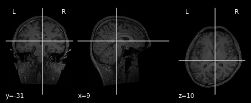
plot_anat(anat_T1)
<nilearn.plotting.displays._slicers.OrthoSlicer at 0x7f682c8aea58>
plot_anat(anat_T2)
/home/jpauli/miniconda3/envs/neuro_ai/lib/python3.7/site-packages/nilearn/image/resampling.py:545: UserWarning: Casting data from int32 to float32
  warnings.warn("Casting data from %s to %s" % (data.dtype.name, aux))
<nilearn.plotting.displays._slicers.OrthoSlicer at 0x7f6813ccd470>
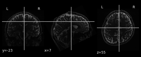
We have two seperate images. The first plot is of the anatomical image of subject one. Important to note is, that we are looking at a T1 weighted image. This results in tissues, that are rich of fat, are highlighted. The second plot is also a anatomical image, taken during the first imagery session of subject one. This is a T2 weighted image, meaning both fat and water is highlighted.
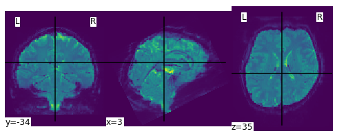
path_func_img = '/home/jpauli/ds001506/sub-01/ses-imagery01/func'

fmri_img = os.path.join(path_func_img ,'sub-01_ses-imagery01_task-imagery_run-01_bold.nii.gz')
from nilearn.image import mean_img
mean_img = mean_img(fmri_img)
plot_img(mean_img)
<nilearn.plotting.displays._slicers.OrthoSlicer at 0x7f6813c0a908>
2.1 Inspection of event file and meta data#
Now its time to inspect the events.tsv and the .json file. The event file tells us for example which stimuli (category_id) was presented at which timestamp (onset) and for how long (duration). The unit for this information is in seconds. Also the event file contains the column Evaluation. It runs from 5 (very) to 1 (could not recognize) and indicates how vivid the mental imagery was for the participants.
import pandas as pd
events=pd.read_csv('/home/jpauli/ds001506/sub-01/ses-imagery01/func/sub-01_ses-imagery01_task-imagery_run-01_events.tsv',sep='\t')
events
| onset | duration | trial_no | event_type | category_id | category_name | category_index | response_time | evaluation | |
|---|---|---|---|---|---|---|---|---|---|
| 0 | 0.0 | 32.0 | 1.0 | -1 | NaN | NaN | NaN | NaN | NaN |
| 1 | 32.0 | 4.0 | 2.0 | 1 | 1976957.0 | n01976957 | 7.0 | 44.967050 | 4.0 |
| 2 | 36.0 | 8.0 | 2.0 | 2 | 1976957.0 | n01976957 | 7.0 | 44.967050 | 4.0 |
| 3 | 44.0 | 3.0 | 2.0 | 3 | 1976957.0 | n01976957 | 7.0 | 44.967050 | 4.0 |
| 4 | 47.0 | 1.0 | 2.0 | 4 | 1976957.0 | n01976957 | 7.0 | 44.967050 | 4.0 |
| ... | ... | ... | ... | ... | ... | ... | ... | ... | ... |
| 101 | 432.0 | 4.0 | 27.0 | 1 | 1943899.0 | n01943899 | 6.0 | 445.498226 | 2.0 |
| 102 | 436.0 | 8.0 | 27.0 | 2 | 1943899.0 | n01943899 | 6.0 | 445.498226 | 2.0 |
| 103 | 444.0 | 3.0 | 27.0 | 3 | 1943899.0 | n01943899 | 6.0 | 445.498226 | 2.0 |
| 104 | 447.0 | 1.0 | 27.0 | 4 | 1943899.0 | n01943899 | 6.0 | 445.498226 | 2.0 |
| 105 | 448.0 | 6.0 | 28.0 | -2 | NaN | NaN | NaN | NaN | NaN |
106 rows × 9 columns
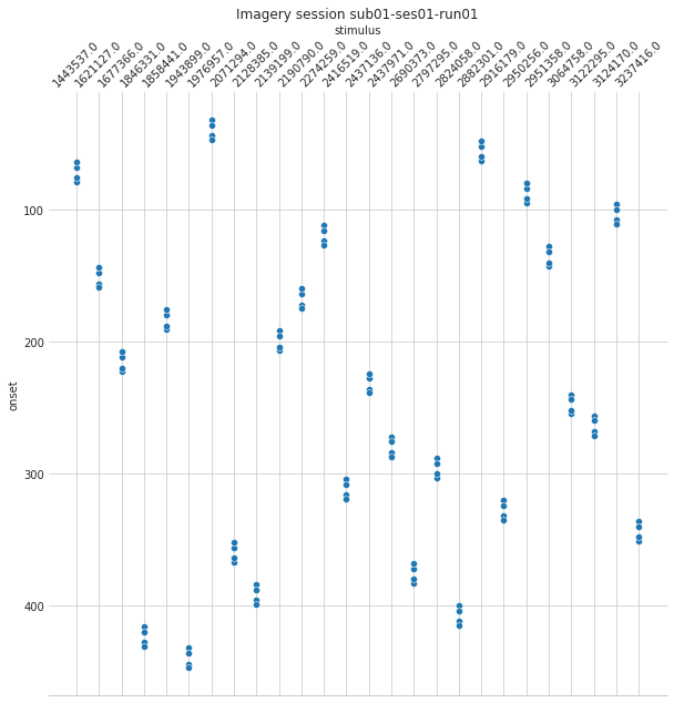
We are also interested in how many unique image categories were used in the experiment, so we use the following command to inspect this:
events.sort_values(by=['category_id'], inplace=True,ascending=True) #sort values, because values are also sorted in design matrix.
categories = events['category_id']
categories_no_nan = categories.dropna()
print('we are dealing with {} categories'.format(len(categories_no_nan.unique())))
we are dealing with 26 categories
import matplotlib.pyplot as plt
%matplotlib inline
plt.style.use('seaborn-whitegrid')
cat_string = [None]*106

for idx, x in enumerate(categories_no_nan):
    cat_string[idx] = str(x)
events['stimulus'] = cat_string
import seaborn as sns
plt.figure(figsize=(10,10))
g=sns.scatterplot(data=events, x='stimulus', y='onset')
sns.despine(left=True)
g.invert_yaxis()
g.xaxis.tick_top()
g.xaxis.set_label_position('top')
plt.xticks(rotation=45);
plt.title('Imagery session sub01-ses01-run01');
import json
with open('/home/jpauli/ds001506/sub-01/ses-imagery01/func/sub-01_ses-imagery01_task-imagery_run-01_bold.json') as json_file:
    json_data = json.load(json_file)
json_data
{'Manufacturer': 'SIEMENS',
 'ManufacturersModelName': 'Verio',
 'MagneticFieldStrength': 3.0,
 'FlipAngle': 80.0,
 'EchoTime': 0.043,
 'RepetitionTime': 2.0,
 'SliceTiming': [0.0,
  1.0575,
  0.1075,
  1.1625,
  0.2125,
  1.2675,
  0.3175,
  1.375,
  0.4225,
  1.48,
  0.53,
  1.585,
  0.635,
  1.6925,
  0.74,
  1.7975,
  0.845,
  1.9025,
  0.9525,
  0.0,
  1.0575,
  0.1075,
  1.1625,
  0.2125,
  1.2675,
  0.3175,
  1.375,
  0.4225,
  1.48,
  0.53,
  1.585,
  0.635,
  1.6925,
  0.74,
  1.7975,
  0.845,
  1.9025,
  0.9525,
  0.0,
  1.0575,
  0.1075,
  1.1625,
  0.2125,
  1.2675,
  0.3175,
  1.375,
  0.4225,
  1.48,
  0.53,
  1.585,
  0.635,
  1.6925,
  0.74,
  1.7975,
  0.845,
  1.9025,
  0.9525,
  0.0,
  1.0575,
  0.1075,
  1.1625,
  0.2125,
  1.2675,
  0.3175,
  1.375,
  0.4225,
  1.48,
  0.53,
  1.585,
  0.635,
  1.6925,
  0.74,
  1.7975,
  0.845,
  1.9025,
  0.9525],
 'MultibandAccelerationFactor': 4,
 'TaskName': 'imagery'}
The json file tells us about the meta data associated with this file. This includes the manufacter, the signal strengh of the magnetic field in tesla, the slicing time and even the respective task name.
3.0 Datamanagment: Data modelling#
Please follow the jupyter book to continue.